Introduction
A backtest is a claim about a counterfactual: had this rule been run on this history, it would have earned this return stream. The claim is only as good as its respect for the arrow of time. Look-ahead bias—letting the simulated decision at bar \(t\) depend on information realized at or after \(t\)—breaks the counterfactual at its root, and unlike overfitting it does not require many trials or a hostile optimizer: a single misplaced index inflates performance deterministically, on the first run, with no warning in the equity curve. The gross forms (training on the test set, using tomorrow’s close) are caught in review. The subtle forms are not: an off-by-one in the fill, a feature standardized over the whole sample, a smoother that happens to be centered. Each is one line, each passes a glance, and each silently converts noise into a track record.
This paper measures how much. We are not the first to warn about look-ahead bias—it is a fixture of every serious treatment of backtesting [1, 2, 13]—but the warnings are almost always qualitative. How many units of Sharpe does a specific leak buy? Is the inflation an all-or-nothing artifact or a gradient? Does it depend on the channel through which the future enters, and if so how much? These questions have answers only when the ground truth is known by construction, which real data never offers. We therefore build a synthetic world in which the true, causally tradable edge is exact, run one honest pipeline and three single-line leaks on the same \(4{,}000\) histories, and read the inflation directly off the gap to truth.
A self-audit, not an indictment.
The first and largest leak we study—booking the position on the same bar that generated the signal—is not a hypothetical. It is the exact bug we shipped in our own parameter-search benchmark.1 The fix was a one-character change to an array index, and it reversed the sign of the conclusion. That experience is the reason this paper exists, and it frames everything that follows: the leaks we dissect are the ones a careful practitioner actually writes by accident, and our aim is to price them, detect them, and—where the honest answer is that a particular leak is harmless—say so plainly.
Contributions.
A reproducible framework in which a one-parameter momentum strategy is run against a known, causally tradable edge, so the exact inflation of any look-ahead form is the measured Sharpe minus the honest-executable truth (Section 3). Two ground truths (a no-edge null and a small real edge), three surgical leaks, \(4{,}000\) seeds each, fully deterministic.
The first dose-quantified measurement of the canonical same-bar fill: it manufactures \(+14.79\) annualized Sharpe from pure noise, and a captured-fraction sweep shows the leak is a smooth gradient (Sections 4.1).
A channel-specificity result. A one-bar centered indicator peek inflates Sharpe by \(+5.50\) from noise, but whole-series normalization of a sign rule does not inflate at all (\(-0.10\), an honest negative); leakage magnitude depends on the channel, and we delimit exactly when normalization is and is not benign (Section 4.3).
A false-deployment accounting and a cheap detector: under the same-bar fill \(68.4\%\) of no-edge configurations look deployable yet truly lose; with a real edge the leaks still dominate the measured Sharpe; and a one-bar fill shift exposes every fill-time leak (Sections 4.4–4.5).
Related work
Look-ahead bias and point-in-time discipline.
The hazard is old and named. [13] treats look-ahead and the temporal structure of financial labels as first-class concerns, motivating purged and embargoed cross-validation because naive splits let test-period information leak into training through overlapping, serially correlated labels. [1] place “avoid look-ahead” among the core rules of a machine-learning-era protocol, and asset pricing institutionalized the same discipline as an accounting convention: [5] lag accounting variables by six months so portfolio formation uses only information a real investor could have held. This literature establishes that look-ahead must be avoided; it rarely supplies a controlled measurement of how badly a specific, realistic leak distorts the headline statistic when the truth is known.
Leakage as a machine-learning failure mode.
Outside finance the same failure is studied as data leakage. [11, 12] give the canonical formulation—information about the target that a deployed model could not legitimately use—and catalogue feature-construction, temporal, and preprocessing leaks; [10] document leakage as a driver of the reproducibility crisis across machine-learning-based science, pervasive and frequently undetected. The preprocessing channel we test—standardizing a feature with whole-sample statistics, including the future—is the textbook example: [9:7.10.2] warn that data-dependent preprocessing must sit inside the cross-validation loop, and scikit-learn lists fitting a scaler before splitting as a flagship pitfall [15]. Our normalization leak is exactly this mistake; our contribution is to show that for a sign rule its effect on the headline Sharpe is negligible—a quantitative qualifier the warnings do not provide.
Backtest overfitting and multiple testing.
A large literature quantifies the other way backtests mislead—selection over many trials. [2] show the expected maximum Sharpe over \(N\) random strategies grows without bound; [3] formalize the probability of backtest overfitting, and [4] derive the deflated Sharpe ratio that haircuts an observed Sharpe for the number of trials and non-normality. The data-snooping tradition supplies the testing machinery: the reality check [17], the superior-predictive-ability test [6], stepwise control [14], their application to technical trading rules [16], and the multiple-testing haircut for cross-sectional asset pricing [7, 8]. This machinery is essential but orthogonal to our question: look-ahead inflates a single backtest deterministically, before any search, so deflation for \(N\) trials does not touch it—our null same-bar Sharpe of \(15\) comes from \(N = 1\). The two errors compound (a leak lifts every candidate a search then selects among), but the leak must be measured and removed in its own right, which is what we do here.
Methods
A world with a known, causally tradable edge.
Each synthetic history is generated by an exogenous latent drift and an idiosyncratic shock. The drift is a stationary AR(1) process, \[\begin{equation} g_t \;=\; \phi\, g_{t-1} \;+\; \sqrt{1-\phi^2}\,u_t, \qquad g_0 = u_0, \qquad u_t \sim \mathcal{N}(0,1)\ \text{i.i.d.}, \label{eq:g} \end{equation}\] with persistence \(\phi = 0.95\) and unit stationary variance, and per-bar returns carry that drift one bar later plus noise, \[\begin{equation} r_t \;=\; a\, g_{t-1} \;+\; \sigma\,\varepsilon_t \quad (t \ge 1), \qquad r_0 = \sigma\varepsilon_0, \qquad \varepsilon_t \sim \mathcal{N}(0,1)\ \text{i.i.d.}, \label{eq:r} \end{equation}\] with \(\sigma = 0.01\) and \(\varepsilon \perp u\). Because \(g\) is exogenous (not a function of past returns) there is no feedback, and because the drift at bar \(t\) is set by \(g_{t-1}\), a forecaster who has tracked \(g\) has a genuine, strictly causal one-bar-ahead edge. The amplitude \(a\) is the only knob on the edge: at \(a = 0\) there is nothing to find (the null); at \(a = 0.0011\) there is a small, real, tradable edge (the edge truth), calibrated so that the honest pipeline earns an annualized Sharpe of about \(+1.57\).
The strategy and the one honest pipeline.
The strategy reads a single causal feature, the trailing-\(L\) momentum of returns with \(L = 24\), \[\begin{equation} m_t \;=\; \sum_{s = t-L+1}^{t} r_s , \label{eq:mom} \end{equation}\] which both tracks the persistent drift \(g\) (the real edge) and, by including the term \(r_t\), mechanically contains the current bar—the channel the same-bar leak exploits. The honest pipeline takes the position \(s_t = \operatorname{sign}(m_t)\) at the close of bar \(t\) and earns the next bar’s return, charging a one-way fee \(c = 0.00045\) (round-trip \(0.09\%\)) on every change of position: \[\begin{equation} p_t \;=\; s_t\, r_{t+1} \;-\; c\,\lvert s_t - s_{t-1}\rvert , \qquad \mathrm{SR}\;=\; \frac{\overline{p}}{\mathrm{std}(p)}\,\sqrt{A}, \quad A = 8760 , \label{eq:pnl} \end{equation}\] the last factor annualizing hourly bars (\(24 \times 365\)). This is the only causally executable pipeline; every leak below is a single edit to it.
Three surgical leaks.
Each look-ahead form changes exactly one thing and holds everything else equal:
same_bar (a fill-time leak). Book the signal bar instead of the next bar: \(p_t = s_t\, r_t - c\lvert s_t - s_{t-1}\rvert\). The signal \(s_t = \operatorname{sign}(m_t)\) is unchanged and causal; only the execution reads a bar it could not yet have filled. This is the off-by-one of the self-audit. We also sweep its dose: book the convex mix \((1-f)\,r_{t+1} + f\,r_t\) for \(f \in \{0, 0.25, 0.5, 1.0\}\), so \(f = 0\) is honest and \(f = 1\) is the full same-bar leak.
norm_full (a preprocessing leak). Standardize the feature with the whole-series mean \(\mu\) and standard deviation \(\sigma_m\) of \(m\) (both computed over the entire history, using the future), then trade \(\operatorname{sign}\!\big((m_t - \mu)/\sigma_m\big)\); execution stays honest (earns \(r_{t+1}\)). For a sign rule this equals \(\operatorname{sign}(m_t - \mu)\): scaling by \(\sigma_m > 0\) cannot change a sign, and the global mean only shifts the zero threshold.
indicator (a feature-time leak). Smooth the feature with a centered three-tap filter that peeks one bar ahead, \(\tilde m_t = (m_{t-1} + m_t + m_{t+1})/3\), and trade \(\operatorname{sign}(\tilde m_t)\); execution stays honest. The filter is non-causal because \(\tilde m_t\) uses \(m_{t+1}\), which embeds \(r_{t+1}\).
Metrics.
For each leak and truth we report the mean annualized Sharpe over seeds with a \(95\%\) confidence interval and the inflation \(\Delta = \mathrm{SR}_{\text{leak}} - \mathrm{SR}_{\mathrm{honest}}\), paired within seed and tested with a paired \(t\)-test (\(n = 4{,}000\)). The inflation is our primary effect size and is well defined for every leak: it is the leaked Sharpe minus the honest causal sign-rule baseline. We also report a looks-deployable rate \(\Pr(\mathrm{SR}_{\text{measured}} \ge 1)\) against a practitioner bar of annualized Sharpe \(1\). A false-deploy rate—\(\Pr(\mathrm{SR}_{\text{measured}} \ge 1\ \text{and}\ \mathrm{SR}_{\text{honest-exec}} < 0)\), the share of configurations that clear the bar while the same signal executed honestly loses money—is reported only for the same-bar fill, because only an execution-time leak has a clean honest counterpart: the identical causal signal filled one bar later ((4)), so measured and truth genuinely diverge. A feature-side leak has no such counterpart—its honest analog is a different feature (a strictly causal trailing smoother, an expanding-window normalization)—so we quantify those leaks by inflation and by the looks-deployable rate, not by a flip rate (Section 4.4).
Design.
Everything is fixed and disclosed: \(4{,}000\) seeds, \(4{,}000\) bars per history, \(L = 24\), \(\sigma = 0.01\), \(\phi = 0.95\), one-way fee \(0.00045\), annualization \(\sqrt{8760}\), deployable bar \(1.0\), master seed \(20260701\). Returns are
numpy/scipy only; there is no external data
and no unseeded state. The honest pipeline trades actively—turnover is
\(0.184\) position changes per bar
under the null and \(0.169\) under the
edge—so fees are paid in every condition and cannot, by themselves,
explain the sign of any result.
Estimator disclosures.
Three conventions, none of which carries the argument. The per-seed
Sharpe uses the population standard deviation (ddof\(=0\)) while the cross-seed confidence
intervals use the sample standard deviation (ddof\(=1\)); at \(4{,}000\) bars and \(4{,}000\) seeds the difference is
negligible. The leaked PnL is positively skewed (the same-bar fill is
correlated with the bar it books), so the Sharpe ratio is a deliberately
imperfect summary of the very statistic the leak attacks—we report it
because it is the number practitioners read, not because it is the
leak’s natural metric. And with \(n =
4{,}000\) paired seeds the inflation \(t\)-statistics are mechanically enormous
(\(\lvert t\rvert\) in the hundreds);
they establish only that the effect is not sampling noise. The effect
size and its confidence interval, not the \(p\)-value, carry every claim below.
Results
A same-bar fill manufactures a large Sharpe from pure noise, by dose
| Null (\(a = 0\)) | Edge (\(a = 0.0011\)) | |||
| Pipeline | Sharpe [95% CI] | \(\Delta\) (paired \(t\)) | Sharpe [95% CI] | \(\Delta\) (paired \(t\)) |
| honest | \(-0.739\) \([-0.787, -0.691]\) | — | \(+1.573\) \([1.521, 1.625]\) | — |
| same_bar | \(+14.789\) \([14.758, 14.821]\) | \(+15.528\) \((724)\) | \(+15.849\) \([15.816, 15.883]\) | \(+14.276\) \((668)\) |
| norm_full | \(-0.840\) \([-0.888, -0.792]\) | \(-0.101\) \((-13.1)\) | \(+1.458\) \([1.405, 1.510]\) | \(-0.116\) \((-13.8)\) |
| indicator | \(+4.762\) \([4.723, 4.801]\) | \(+5.501\) \((454)\) | \(+6.624\) \([6.581, 6.667]\) | \(+5.050\) \((417)\) |
Table 1 is the headline. Run honestly on a world with no edge, the momentum rule earns an annualized Sharpe of \(-0.739\): it pays fees to trade noise and loses, exactly as it should. Change one thing—book the signal bar \(r_t\) instead of the next bar \(r_{t+1}\)—and the same rule on the same histories reports \(+14.789\). The paired inflation is \(+15.528\) Sharpe units (\(t = 724\), \(p \approx 0\) across \(4{,}000\) seeds), and the confidence interval on the leaked Sharpe (\([14.758, 14.821]\)) does not come within \(15\) units of the honest truth. Nothing about the strategy, the data, or the cost model changed; a single array index converted a money-losing rule into one that, taken at face value, would be among the best track records ever recorded.
The mechanism is transparent. The feature \(m_t\) in (3) contains the term \(r_t\), so \(\operatorname{sign}(m_t)\) is positively correlated with the sign of \(r_t\) by construction; booking \(r_t\) therefore harvests that mechanical correlation instead of forecasting anything. This is why the leak does not need an edge to “work”—it reads the present off its own signal—and why it survives review: the feature is genuinely causal, the bug is one bar downstream in the execution.
The leak is a gradient, not a switch.
A natural defense is that such a gross artifact would be obvious. The dose-response in Table 2 and Figure 1 says otherwise. Booking only a fraction \(f\) of the signal bar—a partial fill, a blended price, a touch of the current bar bleeding into execution—inflates the Sharpe smoothly: at \(f = 0.25\) the null Sharpe is already \(+3.899\), at \(f = 0.5\) it is \(+9.855\), reaching \(+14.789\) at the full leak. There is no threshold below which the leak is safe; one quarter of a bar of look-ahead is worth roughly four and a half Sharpe units here. A small, accidental contamination of the fill price is enough to move a strategy from “discard” to “deploy.”
| Dose \(f\) | Null Sharpe [95% CI] | Edge Sharpe [95% CI] |
|---|---|---|
| \(0.00\) | \(-0.739\) \([-0.787, -0.691]\) | \(+1.573\) \([1.521, 1.625]\) |
| \(0.25\) | \(+3.899\) \([3.847, 3.950]\) | \(+6.410\) \([6.354, 6.467]\) |
| \(0.50\) | \(+9.855\) \([9.806, 9.904]\) | \(+12.201\) \([12.147, 12.256]\) |
| \(1.00\) | \(+14.789\) \([14.758, 14.821]\) | \(+15.849\) \([15.816, 15.883]\) |
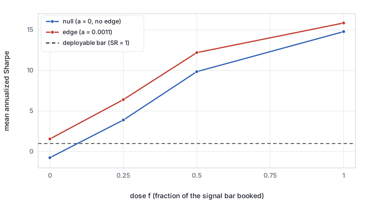
What the leak is: feature–booked-bar overlap, scaling as \(1/\sqrt{L}\)
It is the overlap, not the calendar.
A natural misreading of Section 4.1 is that the hazard is “filling on bar \(t\)” as such. It is not: the hazard is that the feature \(m_t\) and the booked return share the bar \(r_t\). We isolate this with a control that keeps the same-bar fill but removes the overlap. Replace the feature with its lagged form \(m^{-}_t = \sum_{s=t-L}^{t-1} r_s\), which excludes the current bar, and trade \(\operatorname{sign}(m^{-}_t)\); then book the signal bar \(r_t\) exactly as the leak does, and compare to booking \(r_{t+1}\) honestly. Under the null the inflation collapses to \(+0.003\) (\(95\%\) CI \([-0.025, +0.031]\); paired \(t = 0.22\), \(p = 0.82\))—statistically indistinguishable from zero, against \(+15.528\) for the overlapping feature. The off-by-one fill is harmless once the feature no longer contains the bar it books; the entire \(+15\) came from \(\operatorname{sign}(m_t)\) being mechanically correlated with \(r_t\) because \(m_t\) includes \(r_t\). (With a real edge the lagged control inflates by a small \(+0.117\), CI \([+0.090, +0.144]\): when drift is present \(m^{-}_t\) legitimately predicts \(r_t\), so booking it captures a little genuine signal—two orders of magnitude below the overlap artifact.)
The artifact scales as \(1/\sqrt{L}\).
If the leak is overlap, its size should fall as the shared bar’s weight in the feature, \(1/L\), dilutes the signal—and because the Sharpe divides by a return standard deviation that itself shrinks as \(1/\sqrt{L}\), the net scaling is \(1/\sqrt{L}\). Table 3 confirms it: sweeping the look-back over \(L \in \{6, 12, 24, 48, 96\}\) (reduced to \(1{,}500\) seeds per cell), the null same-bar inflation falls from \(+32.43\) to \(+7.65\) while the product \(\Delta\sqrt{L}\) stays nearly flat (\(79.4 \to 74.9\)). The leak is therefore not a fixed “\(+15\) Sharpe” hazard—it is \(\Theta(1/\sqrt{L})\), larger for shorter features. It is also annualization-bound: the headline \(+14.79\) is an annualized figure, while per bar the same-bar null Sharpe is only \(0.158\) (\(= 14.79/\sqrt{8760}\)). The artifact is a small per-bar edge magnified by \(\sqrt{8760}\), exactly as a real edge would be—which is why it is invisible in a single bar and overwhelming in the annualized summary.
| Look-back \(L\) | Null inflation \(\Delta\) | \(\Delta\sqrt{L}\) |
|---|---|---|
| \(6\) | \(+32.425\) | \(79.4\) |
| \(12\) | \(+22.311\) | \(77.3\) |
| \(24\) | \(+15.513\) | \(76.0\) |
| \(48\) | \(+10.840\) | \(75.1\) |
| \(96\) | \(+7.647\) | \(74.9\) |
Channel specificity: an indicator peek inflates, a normalization does not
The two feature-side leaks keep execution honest—both earn \(r_{t+1}\)—and yet land in opposite places (Table 1), which is the paper’s central qualitative point: leakage magnitude is a property of the channel, not a constant.
The indicator peek inflates substantially.
Smoothing the feature with a centered filter that uses \(m_{t+1}\) raises the null Sharpe from \(-0.739\) to \(+4.762\), a paired inflation of \(+5.501\) (\(t = 454\), \(p \approx 0\)). The peek is only one bar wide and only one of three taps, yet it embeds \(r_{t+1}\)—the very bar the position is about to earn—into the signal, so the rule partly decides after seeing its own outcome. A centered moving average is a routine charting primitive; computed in place on a return series and read at the latest bar, it is a look-ahead leak worth five Sharpe units out of nothing.
Whole-series normalization does not.
The same cannot be said for the textbook preprocessing leak. Standardizing the feature with whole-series statistics—the canonical “fit the scaler before the split” mistake [9, 15]—moves the null Sharpe from \(-0.739\) only to \(-0.840\), a paired inflation of \(-0.101\) (\(t = -13.1\), \(p \approx 10^{-38}\)). It is precisely estimated, statistically significant, and economically nil; if anything the leaked rule is slightly worse. The reason is structural and specific: the rule thresholds the feature at zero via \(\operatorname{sign}(\cdot)\), and standardization is an affine map \(m \mapsto (m - \mu)/\sigma_m\) with \(\sigma_m > 0\), so \(\operatorname{sign}((m_t - \mu)/\sigma_m) = \operatorname{sign}(m_t - \mu)\). The scale—the part that genuinely uses the future variance—cannot flip a single sign, and only the global mean \(\mu\) survives, shifting the threshold by a small constant that is as likely to hurt as to help. The future leaks in, but through a door this rule keeps shut.
This benignity is specific to sign rules—do not generalize it.
We state the negative result carefully because it is easy to over-read. Normalization leakage is harmless here only because the decision is a zero-threshold sign. The moment the feature’s magnitude enters the decision—volatility-scaled position sizing, a non-zero or quantile threshold chosen on normalized values, any ranking across assets standardized jointly with the future—the leaked scale and location feed straight into the position, and the same whole-series normalization that is innocuous above would inflate. Our finding is not “normalization leakage is safe”; it is “leakage that cannot reach the decision variable cannot inflate the decision,” of which a sign rule under pure scaling is the clean limiting case. The practical reading is to trace, for each leak, whether the future actually reaches the quantity the rule acts on—which is exactly what separates the \(+5.50\) indicator from the \(-0.10\) normalization.
False deployment and a cheap detector
| Ground truth | looks deployable | false deploy |
|---|---|---|
| Null (\(a = 0\)) | \(100.0\%\) | \(68.4\%\) |
| Edge (\(a = 0.0011\)) | \(100.0\%\) | \(17.4\%\) |
What matters operationally is not the inflated number itself but the decision it drives. Table 4 counts deployments against the practitioner bar of annualized Sharpe \(1\) for the same-bar fill, the one leak with a clean honest counterpart. Every no-edge configuration clears the bar (looks-deployable \(100\%\)), and \(68.4\%\) of them are simultaneously genuine losers—the identical signal, filled one bar later, has a negative Sharpe. This \(68.4\%\) is not independent evidence: because the leak clears the bar in every run, the false-deploy rate is just \(\Pr(\mathrm{SR}_{\text{honest}} < 0)\), the fraction of no-edge histories whose honest backtest happens to lose (the honest null Sharpe has mean \(-0.739\), std \(1.54\)). The leak manufactures no new losers; it dresses every honest losing draw up as deployable. A desk running this pipeline would green-light a portfolio of pure-noise strategies, two-thirds of which lose money live, with full statistical confidence.
The feature-side leaks wave noise over the bar too.
The fill leak is the only one we attach a false-deployment flip rate to, but the feature-side leaks are not harmless—their damage is the Sharpe inflation of Table 1 (\(+5.50\) for the indicator, essentially nil for normalization), and it too generates deployment pressure. Under the null, the indicator peek lifts \(99.9\%\) of no-edge configurations over the deployable bar, and even whole-series normalization clears \(11.9\%\) of them. We deliberately do not report a flip rate for these leaks: because their execution stays honest, the only honest counterpart is a different, strictly causal feature (a trailing smoother, an expanding-window normalization), not the same rule filled differently, so a flip rate would be ill-defined—we let the inflation carry the verdict. The operative point is unchanged: the indicator manufactures a Sharpe that sails over any practitioner threshold out of a world with no edge.
The detector is a one-bar shift.
The same structure that makes the fill leak dangerous also makes it
cheap to catch. Re-run the backtest with every fill shifted forward
exactly one bar and compare. An honest pipeline barely moves (it already
books \(r_{t+1}\)); a same-bar leak
collapses from \(+14.79\) to \(-0.74\)—the out-of-sample sign flips. This
is precisely the diagnostic that exposed the original
bench_search.py bug, and the dose sweep shows it is graded:
a partial leak shrinks under the shift in proportion to the fraction it
was capturing, so the size of the move on shifting fills is itself an
estimate of the leak’s dose. For feature-time leaks the analogous check
is to recompute every feature using only data up to bar \(t\): a strictly causal recomputation of the
same smoother (a one-sided trailing tap in place of the centered one)
performs like the honest baseline, not like the indicator’s inflated
\(+4.76\). Both checks are mechanical,
require no ground truth, and should be standing tests in any backtest
harness.
With a real edge present, leaks still drown out the truth
A tempting hope is that look-ahead matters only in the null—that if a strategy has a real edge, a little leakage merely flatters an already-good number. The edge columns of Table 1 refute it. When the honest pipeline has a genuine, tradable edge (annualized Sharpe \(+1.573\)), the same-bar fill reports \(+15.849\) and the indicator \(+6.624\): the measured Sharpe is inflated to roughly ten times and four times the deployable truth, respectively. The inflation is nearly as large as in the null (\(+14.276\) and \(+5.050\)), because the leak’s contribution is mechanical and adds on top of whatever real edge exists. The practical consequence is that the measured Sharpe is uninformative about skill: a reading of \(15\) is consistent with a worthless rule under a full same-bar leak and with a genuinely good rule under the same leak, and nothing in the number distinguishes them. Even with a real edge, \(17.4\%\) of runs under the same-bar fill clear the deployable bar while the identical signal filled honestly is negative (Table 4)—the edge is real on average but noisy per history, and the leak promotes the unlucky-but-honestly-negative draws all the same. Skill does not immunize a backtest against look-ahead; it only raises the floor the leak builds on.
Discussion
Price the leak, then the search.
The overfitting literature [2–4] teaches us to deflate a Sharpe for the number of trials behind it. Look-ahead bias sits logically before that step and is immune to it: our null same-bar Sharpe of \(14.79\) comes from a single configuration (\(N = 1\)), with nothing to deflate. Worse, the two errors compound—a fill leak lifts every candidate in a search, so a deflated-Sharpe gate downstream is choosing among uniformly inflated candidates and will still deploy. Order of operations matters: establish that the pipeline is causal (shift the fills, causalize the features, watch the sign) before trusting any multiple-testing correction. A deflated Sharpe computed on a leaked backtest is a precise answer to the wrong question.
Channel-specificity is the actionable lesson.
The spread in Table 1—\(+15.5\) for the same-bar fill, \(+5.5\) for the indicator peek, \(-0.1\) for normalization—means a flat “avoid look-ahead” is too coarse to act on. What predicts a leak’s damage is whether the future reaches the quantity the rule actually uses: the fill leak puts it directly into the booked return; the indicator puts \(r_{t+1}\) into the signal; the normalization puts it only into a scale a sign rule discards. Auditing a pipeline is tracing data flow from each future-touching computation to the decision variable, not pattern-matching on the word “normalize.” This connects to purged cross-validation [13]: purging removes the channel by which test-period labels reach the training decision, and where that channel is already closed (our sign rule under scaling) the protection is, correctly, slack. It is the same idea as the accounting-lag convention of [5], and the dose result shows why the lag must be exact: a quarter-bar of look-ahead already buys multiple Sharpe units, so “close enough” alignment is not close enough.
Limitations
Our world is synthetic and deliberately simple: Gaussian shocks, a single exogenous AR(1) drift, a constant volatility, and a frictional but stylized cost model (a fixed per-turn fee, no slippage, spread, or market impact). Real returns have fat tails, volatility clustering, and microstructure that could change every magnitude here, though not the direction of a fill-time leak, which is mechanical. The strategy is a one-dimensional, zero-threshold sign rule on a single asset; the benign normalization result is, as we stress, specific to that sign structure and would not survive magnitude-based sizing, non-zero or data-chosen thresholds, or cross-sectional standardization—exactly the cases a sequel should measure. The three leaks are each a single, clean departure; real bugs often combine several, and interactions are out of scope. Most important, the headline magnitudes are not universal constants: the same-bar inflation scales as \(\approx 1/\sqrt{L}\) in the feature look-back (Table 3, \(+32\) at \(L = 6\) down to \(+8\) at \(L = 96\)) and as \(\sqrt{8760}\) in the annualization (per bar it is only \(0.158\), not \(14.79\)), so a desk on a different bar frequency, look-back, or annualization factor should expect a different headline number for the identical bug. These figures should be read in Sharpe units and as multiples of the honest truth, with the \(L\)- and annualization-dependence in mind, not transplanted as constants. Finally, we study detection only through the fill-shift and causal-recompute checks; we do not test how often practitioners actually run them, which is the human half of the problem.
Conclusion
We measured, against a known ground truth, how much three realistic look-ahead leaks inflate a backtest’s headline Sharpe. A same-bar fill—the off-by-one we once shipped ourselves—manufactures a \(+14.79\) annualized Sharpe out of pure noise, with a smooth dose-response that offers no safe threshold; a one-bar centered indicator peek manufactures \(+4.76\); and whole-series normalization of a sign rule manufactures essentially nothing (\(-0.10\)), an honest negative result that holds only because scaling cannot flip a sign. Under the fill leak every no-edge configuration looks deployable and two-thirds truly lose; and a genuine edge gives no protection, because the leak’s inflation is mechanical and stacks on top of skill, leaving the measured Sharpe unable to tell the two apart. The remedy is order-of-operations and data-flow discipline: prove the pipeline causal—shift the fills one bar, recompute features causally, and require the out-of-sample sign to survive—before deflating for trials or trusting any number a backtest reports. Look-ahead bias is not an exotic failure; it is a one-line edit away at all times, and the only defense that scales is to make its detector a standing test.
Reproducibility.
Every result is deterministic given the released master seed (\(20260701\)). The command
run_all.py regenerates results.json;
check_paper_numbers.py verifies that every number quoted in
this paper matches that file to its printed precision; and the test
suite re-runs a small version of the simulation and asserts the
qualitative invariants. The generative model, the honest pipeline, the
three leaks, and the analysis are released as open source.
In an earlier walk-forward parameter-search harness of ours (
bench_search.py), fills were initially booked on the same bar that produced the signal. Moving execution to the next bar’s open (open[i+1]) flipped the out-of-sample verdict of a Sobol/quasi-random search from systematically negative to systematically positive—the search had been “finding” edges that were nothing but the same-bar fill reading its own signal bar. That bug is the motivation for this study; the experiments below are a controlled audit of our own pipeline, not an attack on a third party.↩︎